In statistics and machine learning, logistic regression is a type of probabilistic classification model. An example of a classification problem is to label an email as either “spam” or “not spam”. Another example is to check if a student based on their score on multiple entrances exams are either “admitted” or “not admitted” to a college. As such, logistic regression is used to predict a binary label  to each instance of a data set, where each point is labeled either as
  which represents a negative label such as not admitting a student, or
  which represents a positive label such as admitting a student. Ultimately what logistic regression tries to do is to solve for a threshold that states if the data is of one label or the other. A classifier has an output function, this is written as
  which takes the input values of
  and gives a numerical output that is normalized between 0 and 1. estimates the probability that on an input . We then compare this to the threshold
  (the threshold can be set to any number, 0.5 is a good pick). This gives us our logistic regression classifier:


In logistic regression we use the logistic function to calculate the output because it can take an input with any value $\latex x$ from negative to positive infinity, whereas the output always takes values between zero and one. It is defined by the sigmoid function  . Below we see the logistic function plotted:
  Going back to our school example for a students grades on two exams, if our classifier gave the following output
  , what does it mean? It means that our student has 70% chance of being admitted, and according to our threshold 0.5 has been admitted. More formally we can say
  which states that the output is equal to the probability that , given , parametrized by
  . Note also that
  . We see here the variable , what is that? Well is a parameter that weighs the input x to define the decision boundary. Now you may say, wait a minute what’s a decision boundary, isn’t that the threshold? Let’s explain what they are. First off we need to change a bit what is. We know it is the input variable that we use as a training example for classifying. But as a training example x may have many features such as being the two scores from our school example. As such we say that that one training example is composed of the following features
  where
where  is the number of features of the training example. For the school case we have
  or
or  . Okay now we have our features defined, how do we pass them through the logistic function to get a classification by our decision rule? Do we pass them in one by one? No we multiple them all by a weighting parameter and then sum them all together as such
  . We then have
  where
where  is the logistic function. In linear algebra this can be written as
  where
where  is the transpose of the matrix of theta’s which multiplies a matrix of x’s. The output of
  is a scalar value that is checked against the threshold
  in our decision rule above. Okay good so far but what is a decision boundary? Well it is a way to imagine our decision rule in a visual way. We define the decision boundary as a line by . To better understand this, let’s go to the school example. Below is a plot. Every point in the plot represents a student. The coordinates of the points
  represent our two features which are the two scores
  the student got on two entrance exams where
  . The blue line is our decision boundary defined by
  . If a student got an output
  it means their scores where above the line and thus classified as having been admitted into college and vice versa if their output was below the decision boundary.
  Something look familiar? It should! The decision boundary as stated before is the equation to a line where
  . The equation to a line is defined as
  where
where  is the slope and
  is the intercept. I’ll leave it to you as an exercise to see how is similar to . Now it is possible to define even more complex decision boundaries for more complicated data examples such as:
 Here we have
  which if you remember your geometry is also the equation to a circle. Did I forget something? Holy cow I did we forgot to show how you actually choose the values of ! This requires a bit more explanation of what a cost function is and how you minimize it by gradient descent to get the values of . Keep a look out for a post on Cost Functions.
 Going back to our school example for a students grades on two exams, if our classifier gave the following output
 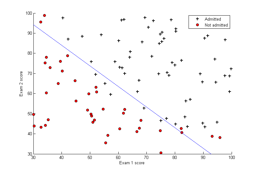 Something look familiar? It should! The decision boundary as stated before is the equation to a line where
  Here we have